GENOME PIXELIZER 2D PLOTTER
PROGRAM DESCRIPTION
GenomePixelizer 2D plotter (or genoPix2D) generates images (actually
interactive canvases) of genomic similarity dot plots, in which each "dot"
indicates similarity between a pair of genes. Diagonal runs of dots
generally indicate collinearity in the genomic regions being compared.
The program can compare large (chromosome-scale or even eukaryotic
genome-scale) genomic regions, and can produce PostScript output of the
dot plots.
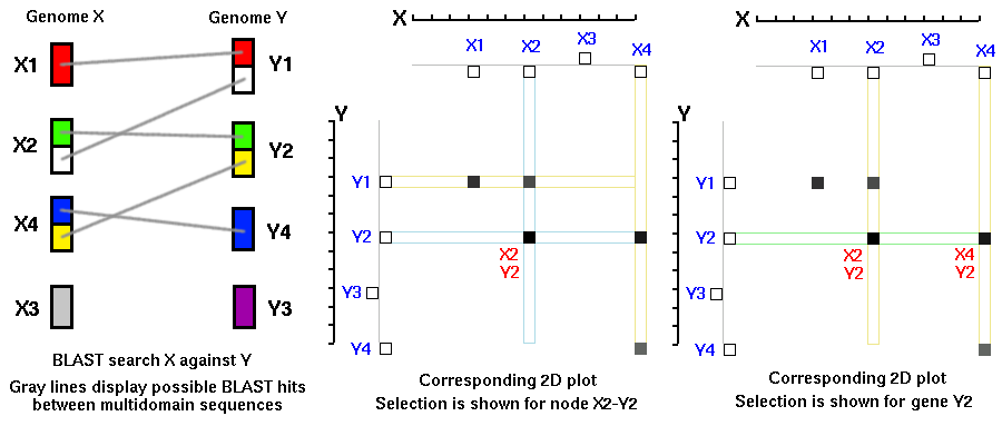
One group of genes (on the X-axis) is compared to another group of genes
(on the Y-axis). If there is a match (similarity) above a defined cutoff
value between a pair of genes (Xi,Yj) then a dot is placed on the 2D plot
with corresponding coordinates (Xi,Yj).
             Xi     Xk    Xp
           +------------------> X axis
           | .      .     .
           | .      .     .
        Yj |.*      .     .
           |        .     .
           |        .     .
        Ym |........*     .
           |              .
        Yq |..............*
           V
          Y axis
                    Figure 1
For example (Figure 1), pairs of genes Xi-Yj, Xk-Ym, Xp-Yq will result in
three dots plotted on 2D graph. If the order of the genes (Xi-Xk-Xp) in
genome X is the same as the order of the genes (Yj-Ym-Yq) in genome Y, then
the plotted dots will form a diagonal. If the order of the genes is
different for both genomes, then the dots will most likely form, random
patterns.
Thus, by identifying diagonals on 2D dot plots it is possible to identify
'syntenic' regions between two different genomes or two chromosomes within
genomes. 'Synteny' means 'same thread' (or ribbon), a state of being
together in location.
The idea of diagonal plots is not new. A search of http://www.google.com/
for keywords
"genome, diagonal, plot"
can find thousands web links to
different programs, published papers and unpublished data to this subject.
What is new in the GenomePixelizer 2D plotter:
1. Images on canvas are not static. They are interactive, and every dot
(element) is associated with corresponding gene annotations that are
searchable by gene ID.
2. A different color scheme can be assigned to every dot (element)
interactively (the "Node painter" function). The "canvas editor" function
allows a user to finish a project by adding custom text labels and simple
graphics.
3. Genes with "hits" (similarity) to other genes, so called "plotted" pairs,
and genes without matching pairs, so called "unplotted" genes, are displayed
in two distinct groups.
4. Zoom-in functionality. By specifying genome coordinates, it is possible
to select regions of interest and display them in a new scale.
5. Scalability. Program can generate canvases and corresponding PostScript
images of very large size (6 feet x 6 feet is not a limit).
6. The program comes with a BLAST parser that generates Matrix files
automatically from BLAST search results.
7. GenomePixelizer 2D plotter is a cross-platform desktop application. It
runs on any computer supporting Tcl/Tk interpreter
(http://tcl.activestate.com)
INPUT FILES
Two input files are required: a "Matrix" file (containing BLAST hit
information), and a "Coords" file (containing gene coordinates). A third
file, with gene annotations, is optional.
The "matrix file" contains identity scores for pairs of genes:
column 1: gene ID in genome A;
column 2: gene ID in genome B;
column 3: identity score for given pair (normalized to [0,1]);
column 4: normalized expectation values;
column 5: alignment length.
Only first three columns of the Matrix file are required by the
GenomePixelizer 2D plotter. All other columns (expectation and alignment
length) are ignored. However, columns with expectation values and alignment
overlap are useful to validate the identity score. The matrix file can be
generated automatically from BLAST output using
tcl_blast_parser_123.tcl
script provided in the "Script" directory.
The "Coords file" contains this information:
column 1: chromosome number;
column 2: gene ID;
column 3: coordinates (position on the chromosome).
Positions on chromosome can be expressed in nucleotides, or in kilobases
(nt/1000), or megabases (nt/1000000, with the decimal portion representing
finer-scale positions). Expressing positions in megabases is recommended
because of compatibility with the previous (original) version of
GenomePixelizer.
Gene coordinates may be derived by parsing corresponding GenBank files or
editing *.ptt (protein translation tables) using an excel-like editor.
For full compatibility with the original version of GenomePixelizer, the
"Coords file" should also contain:
column 4: Watson/Crick gene orientation on chromosome;
column 5: gene color coding.
For details, see:
http://www.atgc.org/GenomePixelizer/GenomePixelizer_Welcome.html
The fourth and fifth columns are not required if you are using the
GenomePixelizer 2D plotter version only.
The annotation file is a tab delimited file with gene IDs in the first
column and their description in the second column. Annotation files may be
derived from fasta headers from corresponding sequence files.
NOTE ABOUT CHROMOSOME NUMBERING:
GenoPix_2D_Plotter reads and understands chromosome IDs as strings (not as integers). If your dataset has
more than 9 (nine) chromosomes you should label them as 01 02 03 ... 08 09 10 11 ... and so on. Program
does not work properly sometime if chromosomes are labeled by different way.
PROGRAM INTERFACE AND OPERATION
The current version of GenomePixelizer 2D plotter comes with example data
for the
Arabidopsis thaliana genome.
In the main window at program startup,
there are three entries for input files:
Gene Coordinates File: Matrix/ath_ncbi.coords
Matrix File: Matrix/ath_ncbi.matrix
Annotation File: Matrix/ath_ncbi.annotation
All three corresponding input files are located in the "Matrix"
directory. On some platforms, the full path may need to be entered in these
windows (e.g.
"/Users/yourhome/yourGenoPixDirectory/Matrix/ath_ncbi.coords").
Entries for different canvas parameters are displayed below input files,
they are:
Chr X dir(ection) - selected chromosome will be plotted on X axis
Chr Y dir(ection) - selected chromosome will be plotted on Y axis
Start X: 0, End: END
Start Y: 0, End: END
these parameters mean that all genes of selected chromosomes will be
plotted on the canvas. It is possible to specify a region of interest in
these entries. In this case only the selected region will be plotted on the
canvas.
Identity cutoff: 0.4 (by default) means that all hits with identity score
40% or better will be plotted on the 2D canvas for selected chromosomes.
Canvas size X: 1000 means that chromosome X will have 1000 pixels width on
the canvas. The Y coordinate for the canvas size will be re-calculated
automatically, proportionally to X chromosome size.
Size of gene (pixels): 3 means that gene "size" (dot or element) on canvas
will have size 3x3 in pixels.
To run a project you need to click on "Load Data" first. The program will
load data from the Coords file and the Matrix file into the computer
memory. By clicking on "Load Annotation," the program reads the Annotation
file.
After loading the Coords and Matrix data into the memory, you can click
"Plot Canvas". The program should create a canvas and plot the genes and
corresponding BLAST hits on it.
Note about program performance: It may take one or more minutes to plot one
chromosome against another. Performance on Windows machines is slower than
on Linux. Whole genome plotting (for example, all five Arabidopsis
chromosomes against themselves -- more than 27,000 genes and about 100,000
corresponding entries from Matrix file) may take a couple of hours.
Genes are plotted on the X and Y axes.
Each axis consists of two adjacent,
parallel lines, which can carry extra information. The outside line (upper
or left) shows the positions of genes which were not used in the dot plot
comparison, they do not have corresponding entries in Matrix file, while the
inside line (lower or right) shows genes that have matches in the comparison
genomic region above the score threshold.
COLOR SCHEME, NODE PAINTER AND TAG SYSTEM ON CANVAS
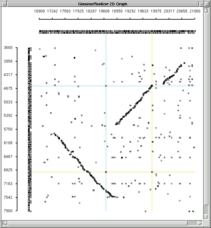
Originally all plotted elements on the canvas are colored proportionally to
identity scores from the Matrix file, with this color scheme:
if "White" color mode is chosen (default):
1.0 - 0.9 - black
0.9 - 0.8 - 90% gray
0.8 - 0.7 - 80% gray
0.7 - 0.6 - 70% gray
0.6 - 0.5 - 60% gray
0.5 - 0.4 - 50% gray
less than 0.4 - 40% gray
canvas background is white
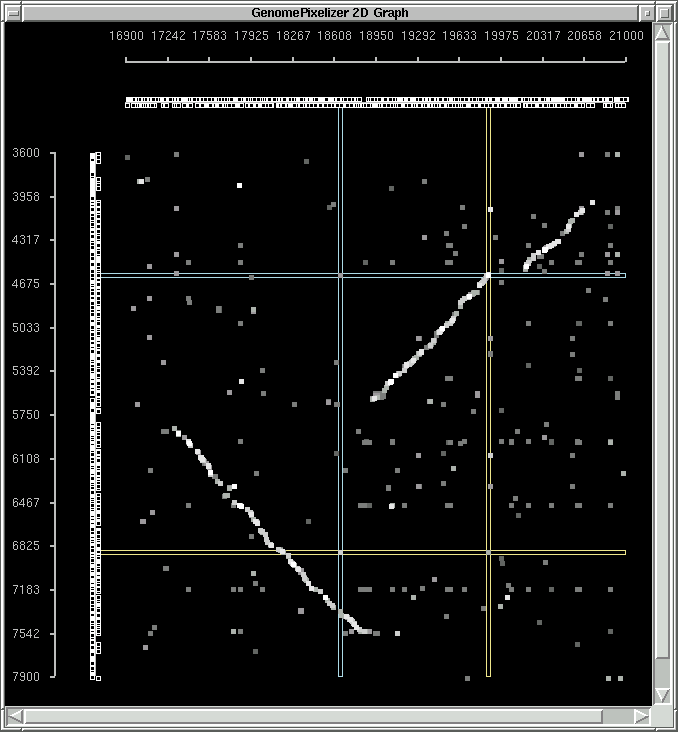
if "Black" color mode is chosen:
1.0 - 0.9 - white
0.9 - 0.8 - 10% gray
0.8 - 0.7 - 20% gray
0.7 - 0.6 - 30% gray
0.6 - 0.5 - 40% gray
0.5 - 0.4 - 50% gray
less than 0.4 - 60% gray
canvas background is black
You can check the examples of "white mode"
and "black mode".
Each element being plotted on the 2D canvas has three IDs or tags. These
tags permit searching the canvas interactively for particular elements
(genes). There is a unique tag for every element. For example if gene "A"
has a hit to gene "B" then a unique tag "A_B" or "B_A" is assigned to
corresponding element. This allows finding the unique elements on the
canvas that correspond to any given gene pair.
If gene "A" has hits to genes "B", "C" and "D" then redundant tag "A" is
assigned to every element in a given set. For example: all dots "A_B",
"A_C" and "A_D" will have tag "A". This allows searching the canvas for all
elements with hits to gene "A".
The "Node painter" function allows a user to perform the search described
above. By clicking on the Node painter, a new window should appear.
Different groups of genes of interest are listed in separate files in the
directory "Group". They contain just gene IDs in a one column file format.
It is possible to reset the color scheme on the canvas back to gray scale
by pressing the button "Color Reset".
Several examples are contained in this distribution: group1 contains IDs of
putative resistance genes, group2 - cytochrome P450, group3 - putative
LRR-protein kinases, group4 - retrotransposon like elements, group5 - all
kinases detected by a HMM model, group6 - Leucine Rich Repeats. By clicking
on the "paint" button for a corresponding group, all elements on the canvas
that have redundant IDs for a given group will be painted in the selected
color. For example, if user clicks on the paint button of group 1, then all
elements (nodes) on the 2D plot will be painted in red if these have BLAST
hits to any resistance gene from the group1 file.
The "diagonal" group is a special group of the Node painter. It permits
displaying elements that have been identified as members of "diagonal"
features (syntenic regions). The group file that contains diagonal
groups has two columns with gene IDs. Each node will be painted according
to the pair of IDs in this file. For example, if line of diagonal group
contains IDs "A" and "B" the only element(s) which will be painted on
canvas are those that have the unique tag "A_B" or "B_A". Also, all genes
on the X and Y axes with tags "A" and "B" will be painted. The diagonals in
this distribution were identified using the DiagHunter perl script by
Steven Cannon. DiagHunter should be included in the Scripts directory, and
is also available via
http://www.tc.umn.edu/~cann0010.
MOUSE CLICKS, EVENTS BINDINGS, AND THE CANVAS EDITOR
A mouse click on any plotted element on the 2D canvas will generate blue
lines that cross on the selected element. Genes with hits to the selected
element will be highlighted with intersecting yellow lines. By mouse click
on genes plotted on X or Y axes green line should appear if gene has hit(s)
to another gene(s). Again, yellow lines crossed with green line indicate
positions for hits to selected gene.
A mouse click will also give annotation information for the selected element
in the "Annotation window," as well as gene IDs and their coordinates in the
"Gene IDs" window.
By using "Canvas Editor" it is possible to add simple graphical labels and
text to the canvas. It is possible to remove all labels with an active tag
by pointing mouse over element and holding "Shift" key with mouse click.
When the "Canvas Editor" window is open, point mouse cursor over any gene or
plotted pair, hold "Control" key and press mouse button, this action will
print gene IDs corresponding to selected element. Removing labels is possible
via holding "Shift" key and mouse click.
SEARCH BY GENE ID OR BY KEYWORD
Canvas is searchable for particular elements (genes) by gene ID or by keyword.
Search by keyword is available only in the case if an "Annotation File" is
loaded into computer memory. To search by gene ID type in the gene ID entry
window ID of the gene you like to find. Search will be successful if the
corresponding gene has been plotted on 2D canvas (it means it has BLAST hit(s)
within specified identity cutoff). In this case a green line on 2D canvas will
point to selected gene on X or Y axes and crossed yellow lines will highlight
all BLAST hits to that selected gene.
"Search by keyword" entry window is located on the bottom of "Annotation
Window". Search by keyword will perform search of annotation description
lines and will paint (highlight) all genes and corresponding BLAST hits with
the color scheme defined in "Canvas Editor" for graphical elements.
You can reset color back to gray scale by clicking on button "Color Reset"
from "Node Painter" window.
ZOOM IN FUNCTIONALITY
It is possible to select and display a region of interest in greater
detail. For example, for default example data set (the Arabidopsis thaliana
genome) select:
Chr X dir: 1 X Start: 19.1 X End: 23.4
Chr Y dir: 1 Y Start: 2.1 Y End: 6.3
Canvas Size X: 600
Then click "Plot Canvas". A canvas with only the selected region for the
given pair of chromosomes should appear, displaying one of the duplicated
regions of the Arabidopsis genome.
SAVING THE RESULTS OF YOUR WORK
Clicking on the button "Save as PostScript" will generate a PostScript file
with the selected filename.
DEFAULT DATA SET
The default data set represents the
Arabidopsis genome, downloaded from the
NCBI site in January 2003. All protein sequences have been BLAST-ed against
one another, with these options:
blastall -p blastp -F F -d ./ath_ncbi.fasta -i ./ath_ncbi.fasta -o
ath_vs_ath_ncbi_200_hits.blastp.out -e 1e-20 -v 200 -b 200
Results of the BLAST search were parsed by the tcl_blast_parser_123
(see http://cgpdb.ucdavis.edu/BlastParser/Blast_Parser.html ), with default
options. All hits with an expectation value 1e-20 or lower and identity of
40% or higher and an alignment overlap greater than 100 amino acids have
been compiled into the Matrix file (actually this matrix file was generated
automatically by tcl_blast_parser_123). Gene coordinates have been
extracted from the corresponding GenBank files.
Searches for domains (group files 1 through 6) were done using the
hmmsearch program (http://hmmer.wustl.edu).
To display all five Arabidopsis chromosomes at once select the
"x-ath_ncbi.coords" file in the "Gene Coordinates File" entry window.
Change X canvas size to 4000 pixels. Because more than 200,000 elements
will be plotted on canvas it will take a while for the plot to finish.
"x-ath_ncbi.coords" file is almost identical to "ath_ncbi.coords" with
exception that for all chromosomes number 1 was assigned and gene
coordinates were recalculated to form continuous long pseudochromosome.
Identification of duplicated regions in Arabidopsis (in the diagonal group
file) was made using Steven Cannon's DiagHunter perl script. DiagHunter you
can found in the "Scripts" directory, or at
www.tc.umn.edu/~cann0010
FEEDBACK
Feedback and comments are very welcome. Please email to:
Alexander Kozik akozik@atgc.org
GenomePixelizer 2D plotter is under the
GNU public license.
Copyright © 2003 University of California at Davis
|