Suite of Python MadMapper scripts for quality control of genetic markers,
group analysis and inference of linear order of markers on linkage groups.
Visualization and validation of genetic maps
using two-dimensional CheckMatrix heat-plots.
Alexander Kozik, UC Davis Genome Center, R.Michelmore lab
This web page gives a brief description of
CheckMatrix usage - genetic map visualization and validation program
(Part 1);
detailed description how to use MadMapper_RECBIT to group genetic markers into distinct
linkage groups (Part 2);
and inference of linear order of markers on linkage groups
using MadMapper_XDELTA program (Part 3).
MadMapper_XDELTA works in conjunction with MadMapper_RECBIT.
CheckMatrix is used to visualize output of MadMapper scripts.
Part 1
CheckMatrix (py_matrix_2D.py) -
visualization and validation of genetic maps using 2-dimensional heat plots
CheckMatrix is used for visualization and validation of genetic maps.
It can be used for visualization of clustering/grouping results of MadMapper.
Here is a brief description and explanation CheckMatrix input and output files.
Detailed description of CheckMatrix can be found at
http://www.atgc.org/XLinkage/
and
http://www.atgc.org/XLinkage/Genetic_Map_Matrix_Plot_Art.html
CheckMatrix
py_matrix_2D_V248_RECBIT.py
takes as input three files:
1. Pairwise Distance Matrix File
madmapper_test_small.out.pairs_all
pairwise distance matrix file can be generated by
Python MadMapper
from Locus File
       .....................
       GM01    GM07    0.36
       GM01    GM08    0.40
       GM01    GM09    0.48
       GM01    GM10    0.52
       GM01    GM11    0.60
       GM01    GM12    0.68
       GM02    GM01    0.04
       GM02    GM02    0.00
       GM02    GM03    0.08
       GM02    GM04    0.16
       GM02    GM05    0.20
       GM02    GM06    0.24
       .....................
2. Genetic Map File
madmapper_test_small.map.right
(on this example last column reflects the order markers)
       LG      GM01     0
       LG      GM02     1
       LG      GM03     2
       LG      GM04     3
       LG      GM05     4
       LG      GM06     5
       LG      GM07     6
       LG      GM08     7
       LG      GM09     8
       LG      GM10     9
       LG      GM11    10
       LG      GM12    11
3. Locus File (Raw Marker Scores) madmapper_test_small.loc
               1                 10                  20        25
               |                 |                   |         |
       GM01    A A A A A A A A A A A A A A A A B B B B B B B B B
       GM02    A A A A A A A A A A A A A A A B B B B B B B B B B
       GM03    A A A A A A A A A A A A A B B B B B B B B B B B B
       GM04    A A A A A A A A A A A B B B B B B B B B B B B B B
       GM05    A A A A A A A A A A B B B B B B B B B B B B B B B
       GM06    A A A A A A A A A B B B B B B B B B B B B B B B B
       GM07    A A A A A A A A A B B B B B B B B B B B B B B A A
       GM08    A A A A A A A A A B B B B B B B B B B B B B A A A
       GM09    A A A A A A A A A B B B B B B B B B B B A A A A A
       GM10    B A A A A A A A A A B B B B B B B B B A A A A A A
       GM11    B B A A A A A A A A B B B B B B B B A A A A A A A
       GM12    B B B A A A A A A A B B B B B B B A A A A A A A A
by execution of the script with several arguments/options (detailed explanation of options is
here):
$python py_matrix_2D_V248_RECBIT.py madmapper_test_small.out.pairs_all madmapper_test_small.map.right
madmapper_test_small.map.right.xout X Y madmapper_test_small.loc REC NOGRAPH 0.9 LARGE RIL
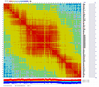
graphical output will be generated:
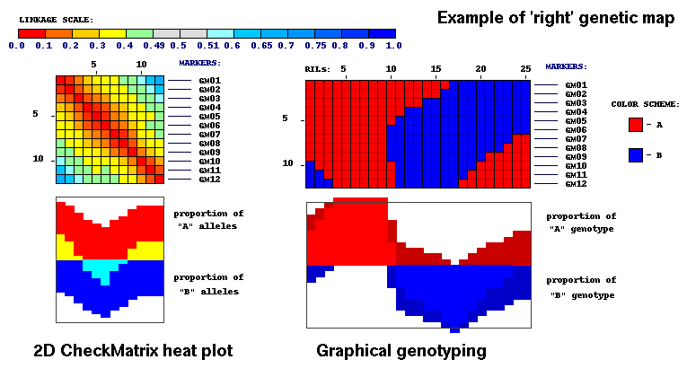
Note, that a good (or 'right') map forms a red diagonal on 2D plot running from left upper corner to the bottom of image.
All colors (and corresponding pairwise scores) display smooth transition from any cell on 2D plot to adjacent cells.
Good map has no 'jumps' in adjacent scores on two-dimensional matrix.
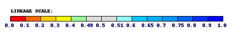
Visualization of the 'right' map above is based on the assignment of different color values
to the pairwise distance matrix data in numerical format:
+--------+--------+--------+--------+--------+--------+--------+--------+--------+--------+--------+--------+--------+
|  ####  |  GM01  |  GM02  |  GM03  |  GM04  |  GM05  |  GM06  |  GM07  |  GM08  |  GM09  |  GM10  |  GM11  |  GM12  |
+--------+--------+--------+--------+--------+--------+--------+--------+--------+--------+--------+--------+--------+
|  GM01  |  0.00  |  0.04  |  0.12  |  0.20  |  0.24  |  0.28  |  0.36  |  0.40  |  0.48  |  0.52  |  0.60  |  0.68  |
+--------+--------+--------+--------+--------+--------+--------+--------+--------+--------+--------+--------+--------+
|  GM02  |  0.04  |  0.00  |  0.08  |  0.16  |  0.20  |  0.24  |  0.32  |  0.36  |  0.44  |  0.48  |  0.56  |  0.64  |
+--------+--------+--------+--------+--------+--------+--------+--------+--------+--------+--------+--------+--------+
|  GM03  |  0.12  |  0.08  |  0.00  |  0.08  |  0.12  |  0.16  |  0.24  |  0.28  |  0.36  |  0.40  |  0.48  |  0.56  |
+--------+--------+--------+--------+--------+--------+--------+--------+--------+--------+--------+--------+--------+
|  GM04  |  0.20  |  0.16  |  0.08  |  0.00  |  0.04  |  0.08  |  0.16  |  0.20  |  0.28  |  0.32  |  0.40  |  0.48  |
+--------+--------+--------+--------+--------+--------+--------+--------+--------+--------+--------+--------+--------+
|  GM05  |  0.24  |  0.20  |  0.12  |  0.04  |  0.00  |  0.04  |  0.12  |  0.16  |  0.24  |  0.28  |  0.36  |  0.44  |
+--------+--------+--------+--------+--------+--------+--------+--------+--------+--------+--------+--------+--------+
|  GM06  |  0.28  |  0.24  |  0.16  |  0.08  |  0.04  |  0.00  |  0.08  |  0.12  |  0.20  |  0.32  |  0.40  |  0.48  |
+--------+--------+--------+--------+--------+--------+--------+--------+--------+--------+--------+--------+--------+
|  GM07  |  0.36  |  0.32  |  0.24  |  0.16  |  0.12  |  0.08  |  0.00  |  0.04  |  0.12  |  0.24  |  0.32  |  0.40  |
+--------+--------+--------+--------+--------+--------+--------+--------+--------+--------+--------+--------+--------+
|  GM08  |  0.40  |  0.36  |  0.28  |  0.20  |  0.16  |  0.12  |  0.04  |  0.00  |  0.08  |  0.20  |  0.28  |  0.36  |
+--------+--------+--------+--------+--------+--------+--------+--------+--------+--------+--------+--------+--------+
|  GM09  |  0.48  |  0.44  |  0.36  |  0.28  |  0.24  |  0.20  |  0.12  |  0.08  |  0.00  |  0.12  |  0.20  |  0.28  |
+--------+--------+--------+--------+--------+--------+--------+--------+--------+--------+--------+--------+--------+
|  GM10  |  0.52  |  0.48  |  0.40  |  0.32  |  0.28  |  0.32  |  0.24  |  0.20  |  0.12  |  0.00  |  0.08  |  0.16  |
+--------+--------+--------+--------+--------+--------+--------+--------+--------+--------+--------+--------+--------+
|  GM11  |  0.60  |  0.56  |  0.48  |  0.40  |  0.36  |  0.40  |  0.32  |  0.28  |  0.20  |  0.08  |  0.00  |  0.08  |
+--------+--------+--------+--------+--------+--------+--------+--------+--------+--------+--------+--------+--------+
|  GM12  |  0.68  |  0.64  |  0.56  |  0.48  |  0.44  |  0.48  |  0.40  |  0.36  |  0.28  |  0.16  |  0.08  |  0.00  |
+--------+--------+--------+--------+--------+--------+--------+--------+--------+--------+--------+--------+--------+
It was an example of visualization of 'good' or 'right' map.
...............
Now we will run CheckMatrix with 'bad' genetic map.
CheckMatrix with 'wrong' marker order (markers GM10 and GM03 are flipped):
       LG      GM01     0
       LG      GM02     1
       LG      GM10     2  ***
       LG      GM04     3
       LG      GM05     4
       LG      GM06     5
       LG      GM07     6
       LG      GM08     7
       LG      GM09     8
       LG      GM03     9  ***
       LG      GM11    10
       LG      GM12    11
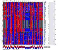
produces following heat plot:
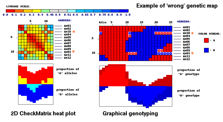
It is easy to notice color distortion on this image. It indicates that map is wrong and has to be fixed.
There are large 'jumps' in adjacent distance matrix values for markers GM03 and GM10.
+--------+--------+--------+--------+--------+--------+--------+--------+--------+--------+--------+--------+--------+
|  ####  |  GM01  |  GM02  |  GM10  |  GM04  |  GM05  |  GM06  |  GM07  |  GM08  |  GM09  |  GM03  |  GM11  |  GM12  |
+--------+--------+--------+--------+--------+--------+--------+--------+--------+--------+--------+--------+--------+
|  GM01  |  0.00  |  0.04  |  0.52  |  0.20  |  0.24  |  0.28  |  0.36  |  0.40  |  0.48  |  0.12  |  0.60  |  0.68  |
+--------+--------+--------+--------+--------+--------+--------+--------+--------+--------+--------+--------+--------+
|  GM02  |  0.04  |  0.00  |  0.48  |  0.16  |  0.20  |  0.24  |  0.32  |  0.36  |  0.44  |  0.08  |  0.56  |  0.64  |
+--------+--------+--------+--------+--------+--------+--------+--------+--------+--------+--------+--------+--------+
|  GM10  |  0.52  |  0.48  |  0.00  |  0.32  |  0.28  |  0.32  |  0.24  |  0.20  |  0.12  |  0.40  |  0.08  |  0.16  |
+--------+--------+--------+--------+--------+--------+--------+--------+--------+--------+--------+--------+--------+
|  GM04  |  0.20  |  0.16  |  0.32  |  0.00  |  0.04  |  0.08  |  0.16  |  0.20  |  0.28  |  0.08  |  0.40  |  0.48  |
+--------+--------+--------+--------+--------+--------+--------+--------+--------+--------+--------+--------+--------+
|  GM05  |  0.24  |  0.20  |  0.28  |  0.04  |  0.00  |  0.04  |  0.12  |  0.16  |  0.24  |  0.12  |  0.36  |  0.44  |
+--------+--------+--------+--------+--------+--------+--------+--------+--------+--------+--------+--------+--------+
|  GM06  |  0.28  |  0.24  |  0.32  |  0.08  |  0.04  |  0.00  |  0.08  |  0.12  |  0.20  |  0.16  |  0.40  |  0.48  |
+--------+--------+--------+--------+--------+--------+--------+--------+--------+--------+--------+--------+--------+
|  GM07  |  0.36  |  0.32  |  0.24  |  0.16  |  0.12  |  0.08  |  0.00  |  0.04  |  0.12  |  0.24  |  0.32  |  0.40  |
+--------+--------+--------+--------+--------+--------+--------+--------+--------+--------+--------+--------+--------+
|  GM08  |  0.40  |  0.36  |  0.20  |  0.20  |  0.16  |  0.12  |  0.04  |  0.00  |  0.08  |  0.28  |  0.28  |  0.36  |
+--------+--------+--------+--------+--------+--------+--------+--------+--------+--------+--------+--------+--------+
|  GM09  |  0.48  |  0.44  |  0.12  |  0.28  |  0.24  |  0.20  |  0.12  |  0.08  |  0.00  |  0.36  |  0.20  |  0.28  |
+--------+--------+--------+--------+--------+--------+--------+--------+--------+--------+--------+--------+--------+
|  GM03  |  0.12  |  0.08  |  0.40  |  0.08  |  0.12  |  0.16  |  0.24  |  0.28  |  0.36  |  0.00  |  0.48  |  0.56  |
+--------+--------+--------+--------+--------+--------+--------+--------+--------+--------+--------+--------+--------+
|  GM11  |  0.60  |  0.56  |  0.08  |  0.40  |  0.36  |  0.40  |  0.32  |  0.28  |  0.20  |  0.48  |  0.00  |  0.08  |
+--------+--------+--------+--------+--------+--------+--------+--------+--------+--------+--------+--------+--------+
|  GM12  |  0.68  |  0.64  |  0.16  |  0.48  |  0.44  |  0.48  |  0.40  |  0.36  |  0.28  |  0.56  |  0.08  |  0.00  |
+--------+--------+--------+--------+--------+--------+--------+--------+--------+--------+--------+--------+--------+
Compare values for marker GM03 (underlined on corresponding column) to its adjacent values.
The difference between these adjacent values is larger (greater) in comparison to 'good' matrix file.
Best map should have smallest difference in adjacent values on 2D matrix overall.
In other words, for the best map total sum of these 'delta'
(difference between adjacent values) should be smallest.
Example of visualization using CheckMatrix of random distribution of genetic markers

Part 2
MadMapper_RECBIT - group analysis and quality control of genetic markers.
We will use DL_RIL_Data.may2001.loc Dean and Lister's
Arabidopsis genotyping data set (locus file)
[ it has raw scores for 1357 markers and was downloaded from
arabidopsis.info web site ]
as an example to demonstrate how to run
Python_MadMapper_V248_RECBIT_012.py
script to solve following problems:
1. Group (cluster) all markers from locus file and assign markers to distinct linkage groups.
2. Select markers for linkage group 4 (as an example) and extract from that group reliable markers
with high quality scores.
3. Then we will go to Part 3 and will try to infer linear order of
selected markers on Arabidopsis linkage group 4.
Python_MadMapper_V248_RECBIT_012.py
script takes as input two files:
1. DL_RIL_Data.may2001.loc locus file with raw marker scores.
2. Dean_Lister_frame.IDs frame work map (optional).
Details about Python_MadMapper_V248_RECBIT_012.py usage can be found by running the script without arguments and
in the README_MADMAPPER_248.txt file;
as well as useful description of previous versions can be found
here
for example:
bash-2.03$ python Python_MadMapper_V248_RECBIT_012.py

   PROGRAM  USAGE:
   MAD MAPPER TAKES 10 ARGUMENTS/OPTIONS IN THE FOLLOWING ORDER:
  (1)input_file[LOC_DATA/MARKER SCORES]          (2)output_file[NAME]
  (3)rec_cut[0.2]          (4)bit_cut[100]       (5)data_cut[25]
  (6)group_file[OPTIONAL]  (7)allele_dist[0.33]  (8)missing_data[50]
  (9)trio_analysis[TRIO/NOTRIO]                  (10)double_cross[3]

   if group_file does not exist just enter [X]

   DEFAULT VALUES:    IN  OUT  0.2  100  25  X  0.33  50  TRIO  3

   TYPE "HELP" FOR HELP [ "EXIT" TO EXIT ] : HELP

              MAD MAPPER ARGUMENTS/OPTIONS - BRIEF EXPLANATION:

       INPUT/OUTPUT FILES:
   [1] - Input File Name  (locus file with raw marker scores)
   [2] - Output File Name (master name [prefix] for 80 or so output files)

       CLUSTERING PARAMETERS (WILL AFFECT CLUSTERING/GROUPING ONLY):
   [3] - Recombination Value (Haplotype Distance) cutoff:  0.20 - 0.25
         (NOTE: TRIO analysis (see below) works with 0.2 rec_cut value only)
   [4] - BIT Score cutoff: 60-1000 [100 is default and highly recommended]
         (Check README_MADMAPPER for BIT Scoring Matrix system and values)
   [5] - Overlap Data cutoff (data_cut): minimum number of scores between
         two markers to be compared to assign pairwise distance

   [6] - Optional Frame Work Marker Map (very useful for clustering analysis
                              to assign new markers to known linkage groups)

       FILTERING PARAMETERS (WILL AFFECT MARKER FILTERING, CREATION OF GOOD
                             NON-REDUNDANT SET OF MARKERS AND TRIO ANALYSIS):
   [7] - Allele Distortion: to filter markers with high allele distortion
   [8] - Missing Data: how many missing scores are allowed per marker

       TRIO (TRIPLET) ANALYSIS -
       FINDING OF TIGHTLY LINKED MARKERS AND THEIR RELATIVE ORDER:
   [9] - TRIO/NOTRIO (If TRIO option is chosen then TRIPLET analysis will
                      take place. Is not recommended to use for large set
                      markers, 1000 or greater)
   [10] - Number of Double Crossovers cutoff value for TRIPLET analysis:
          3 - default for noisy data; 0 is recommended for perfect scores

   CHECK README_MADMAPPER FOR DETAILED DESCRIPTION OF OPTIONS
                           AND OUTPUT FILES FORMATS/STRUCTURE
First Step - Group Analysis - We will run the script with the following options/arguments:
$python Python_MadMapper_V248_RECBIT_012.py DL_RIL_Data.may2001.loc DL_RIL_Data.may2001.xout248 0.2 100 25 Dean_Lister_frame.IDs 0.33 50 NOTRIO 3
Output will be represented by 76 files (find more about the output in the
README_MADMAPPER_248.txt file).
[ Note, that at this time the script was running with "NOTRIO" option ]
At this step we are interested in
DL_RIL_Data.may2001.xout248.x_tree_clust
file only. This file has the information about marker clustering/grouping. From this file we will select
markers belonging to the linkage group 4.
We will analyze DL_RIL_Data.may2001.xout248.x_tree_clust
file using MS Excel to find and highlight (select) a set of markers belonging to the linkage group 4.
DL_RIL_Data.may2001.xout248.x_tree_clust.xls -
tree clustering file in MS Excel format.
Screenshot of the region of interest:
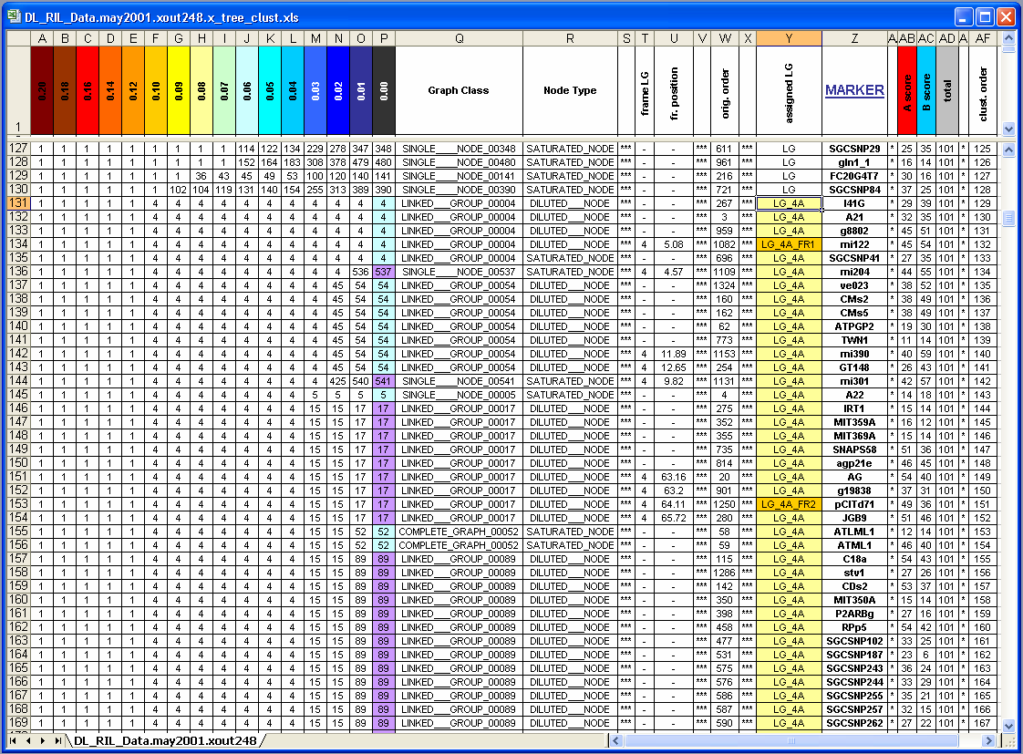
From this group info file we will extract marker IDs belonging to the linkage group 4
DL_RIL_LG4A.tab and create new locus
file DL_RIL_LG4A.loc which contains marker scores for
linkage group 4 only. It has raw scores for 247 markers.
Now we will run Python_MadMapper_V248_RECBIT_012.py again on DL_RIL_LG4A.loc file with "TRIO" option:
$python Python_MadMapper_V248_RECBIT_012.py DL_RIL_LG4A.loc DL_RIL_LG4A.xout248 0.2 100 25 Dean_Lister_frame.IDs 0.33 50 TRIO 3
83 files will be generated. We are interested in the Marker Summary file:
DL_RIL_LG4A.xout248.z_marker_sum
which contains information
about loss of data and allele distortion for each marker, as well as useful information derived from
"TRIO" analysis. From this file we will extract marker IDs
which have "GOOD__MARKER" label (grade) only. It means we will use high-quality markers for further analysis.
These markers have low fraction of data loss and meaningful ratio of "A"/"B" scores (allele distortion).
There are 171 'good' markers in the dataset.
Also, we will need DL_RIL_LG4A.xout248.pairs_all for
further analysis. This file contains pairwise distances for all markers of linkage group 4.
So, from here we are ready to jump to the Part 3 to infer linear order of markers on linkage group 4.
Part 3
MadMapper_XDELTA - inference of linear order of markers on linkage groups using
Minimum Entropy Approach and Best-Fit Extension.
Python_MadMapper_V248_XDELTA_016.py
script infers linear order of markers on a linkage group by analysis of two dimensional matrices of pairwise distances.
MadMapper_XDELTA tries to find the 2D matrix which has minimal total sum of differences between adjacent cells.
The script calculates so called 'delta' for each pair of adjacent cells by subtracting one pairwise score from the
adjacent one. Then it calculates the sum of absolute values of all deltas and chooses that matrix which has a lowest
value. In other words, MadMapper_XDELTA is searching for the matrix with the lowest entropy among a set of
available matrices. Check examples of 'right' and 'wrong' maps from the Part 1 of this web page.
'Right' map has a lower entropy compare to high entropy of 'wrong' map.
All values in a two dimensional matrix of pairwise distances are taken into account even for pairs of unlinked markers.
In other words, contribution of pairwise distances between any pair of markers are equal to find the best map with
lowest entropy. This is the major difference of MadMapper_XDELTA approach in comparison to 'classical' genetic map
programs where scores only for linked markers are considered to construct maps.
Finding of the linear order for N markers has (N!)/2 complexity. For ten markers it is (10!)/2 =
1,814,400 [ almost two million of different orders is available for 10 markers ]. So, we can not check all
available matrices for a set of markers 12 or higher in a real time [ using single CPU of 1 to 5 GHz ].
To minimize a number of matrices to analyze, MadMapper_XDELTA script uses a frame work marker order and tries to
insert all other markers one by one into the frame map calculating 'delta' for each iteration. New map with
lowest delta is selected after each iteration. Run time using this approach does not exceed N x N x N time.
If frame work map is not available, MadMapper_XDELTA can check ALL POSSIBLE COMBINATIONS of orders for up to 10
chosen markers. Then it adds markers one by one from the 'markers to map list'. In this case run time for the script
is (N!)/2 + (M x M x M) where N is a number of frame work markers, M is a number of all markers to map.
Before we run MadMapper_XDELTA with a real set of markers (Arabidopsis linkage group 4 from the Part 2 of this web page)
we will show how to use it and how it works with a smaller example set from the Part 1.
Three input files are required:
1. madmapper_test_small.out.pairs_all [ pairwise distances ]
2. madmapper_test_small.list [ list of markers to map ]
3. madmapper_test_small.frame [ list of frame work markers ]
We will execute the script with the following options:
$python Python_MadMapper_V248_XDELTA_016DD.py madmapper_test_small.out.pairs_all madmapper_test_small.list madmapper_test_small.frame madmapper_test_small.xdelta LG FLEX
As a first step, MadMapper_XDELTA will find the best order for frame work markers [ three markers in madmapper_test_small.frame file ]
and then it will add one by one markers from madmapper_test_small.list file. Calculation of delta for first 18 iterations will
look like:
=============================================
 MATRIX (ALL PAIRS) :  madmapper_test_small.out.pairs_all
 MARKERS  TO  MAP   :  madmapper_test_small.list
 FRAME MARKERS LIST :  madmapper_test_small.frame
 OUTPUT  MAP  FILE  :  madmapper_test_small.xdelta
 MAX FRAME LENGTH   :  12
 FIXED FRAME ORDER  :  FALSE
 LINKAGE GROUP ID   :  LG
 DUMMY DEBUG        :  TRUE
=============================================
=======
GM02    GM06    GM10    ***     1.52    ***     0.5067  ***     1
GM02    GM10    GM06    ***     1.92    ***     0.64    ***     2
GM06    GM02    GM10    ***     1.68    ***     0.56    ***     3
=======
=======
GM03    GM02    GM06    GM10    ***     2.16    ***     0.54    ***     1
GM02    GM03    GM06    GM10    ***     2.0     ***     0.5     ***     2
GM02    GM06    GM03    GM10    ***     2.64    ***     0.66    ***     3
GM02    GM06    GM10    GM03    ***     3.2     ***     0.8     ***     4
=======
=======
GM08    GM02    GM03    GM06    GM10    ***     3.64    ***     0.728   ***     1
GM02    GM08    GM03    GM06    GM10    ***     4.32    ***     0.864   ***     2
GM02    GM03    GM08    GM06    GM10    ***     3.28    ***     0.656   ***     3
GM02    GM03    GM06    GM08    GM10    ***     2.56    ***     0.512   ***     4
GM02    GM03    GM06    GM10    GM08    ***     3.16    ***     0.632   ***     5
=======
=======
GM09    GM02    GM03    GM06    GM08    GM10    ***     4.8     ***     0.8     ***     1
GM02    GM09    GM03    GM06    GM08    GM10    ***     5.92    ***     0.9867  ***     2
GM02    GM03    GM09    GM06    GM08    GM10    ***     4.72    ***     0.7867  ***     3
GM02    GM03    GM06    GM09    GM08    GM10    ***     3.76    ***     0.6267  ***     4
GM02    GM03    GM06    GM08    GM09    GM10    ***     3.12    ***     0.52    ***     5
GM02    GM03    GM06    GM08    GM10    GM09    ***     3.52    ***     0.5867  ***     6
=======
Note that the lowest delta (red) value corresponds to the best 'right' map in each set of iterations.
Finally, the best map for all 12 markers will be generated
madmapper_test_small.xdelta.mad_map_final:
LG  MARKER   POS   #1#     DST1   #2#    DST2   #3#    DST3   #S#    SUMM   #D#   DIFF   STATUS  CLASS
LG    GM01   0     #1#     0      #2#   NNNNNN  #3#   NNNNNN  #S#   NNNNNN  #D#  NNNNNN  NNNNNN  NNNNN
LG    GM02   1     #1#     0.04   #2#    0.08   #3#    0.12   #S#    0.12   #D#   0.0     GOOD   __0__
LG    GM03   2     #1#     0.08   #2#    0.08   #3#    0.16   #S#    0.16   #D#   0.0     GOOD   __0__
LG    GM04   3     #1#     0.08   #2#    0.04   #3#    0.12   #S#    0.12   #D#   0.0     GOOD   __0__
LG    GM05   4     #1#     0.04   #2#    0.04   #3#    0.08   #S#    0.08   #D#   0.0     GOOD   __0__
LG    GM06   5     #1#     0.04   #2#    0.08   #3#    0.12   #S#    0.12   #D#   0.0     GOOD   __0__
LG    GM07   6     #1#     0.08   #2#    0.04   #3#    0.12   #S#    0.12   #D#   0.0     GOOD   __0__
LG    GM08   7     #1#     0.04   #2#    0.08   #3#    0.12   #S#    0.12   #D#   0.0     GOOD   __0__
LG    GM09   8     #1#     0.08   #2#    0.12   #3#    0.2    #S#    0.2    #D#   0.0     GOOD   __0__
LG    GM10   9     #1#     0.12   #2#    0.08   #3#    0.2    #S#    0.2    #D#   0.0     GOOD   __0__
LG    GM11   10    #1#     0.08   #2#    0.08   #3#    0.16   #S#    0.16   #D#   0.0     GOOD   __0__
LG    GM12   11    #1#     0.08   #2#   NNNNNN  #3#   NNNNNN  #S#    NNNNNN #D#  NNNNNN  NNNNNN  NNNNN
OK, it is time for the real set, finally:
Input files [ 'good' markers for Arabidopsis linkage group 4 ]:
1. DL_RIL_LG4A.xout248.pairs_all - pairwise distances
2. DL_RIL_LG4A.list.good - list of markers to map
3. DL_RIL_LG4A.frame - list of frame work markers
$python Python_MadMapper_V248_XDELTA_016.py DL_RIL_LG4A.xout248.pairs_all DL_RIL_LG4A.list.good DL_RIL_LG4A.frame DL_RIL_LG4A.list.xdelta 4 FLEX
Output files:
1. DL_RIL_LG4A.list.xdelta.mad_map_final - final best map
2. DL_RIL_LG4A.list.xdelta.mad_map_log - log file
3. DL_RIL_LG4A.list.xdelta.mad_map_temp -
file with all best maps after each set of iterations
4. DL_RIL_LG4A.list.xdelta.mad_map_xjump - 'deltas' for each set of iterations
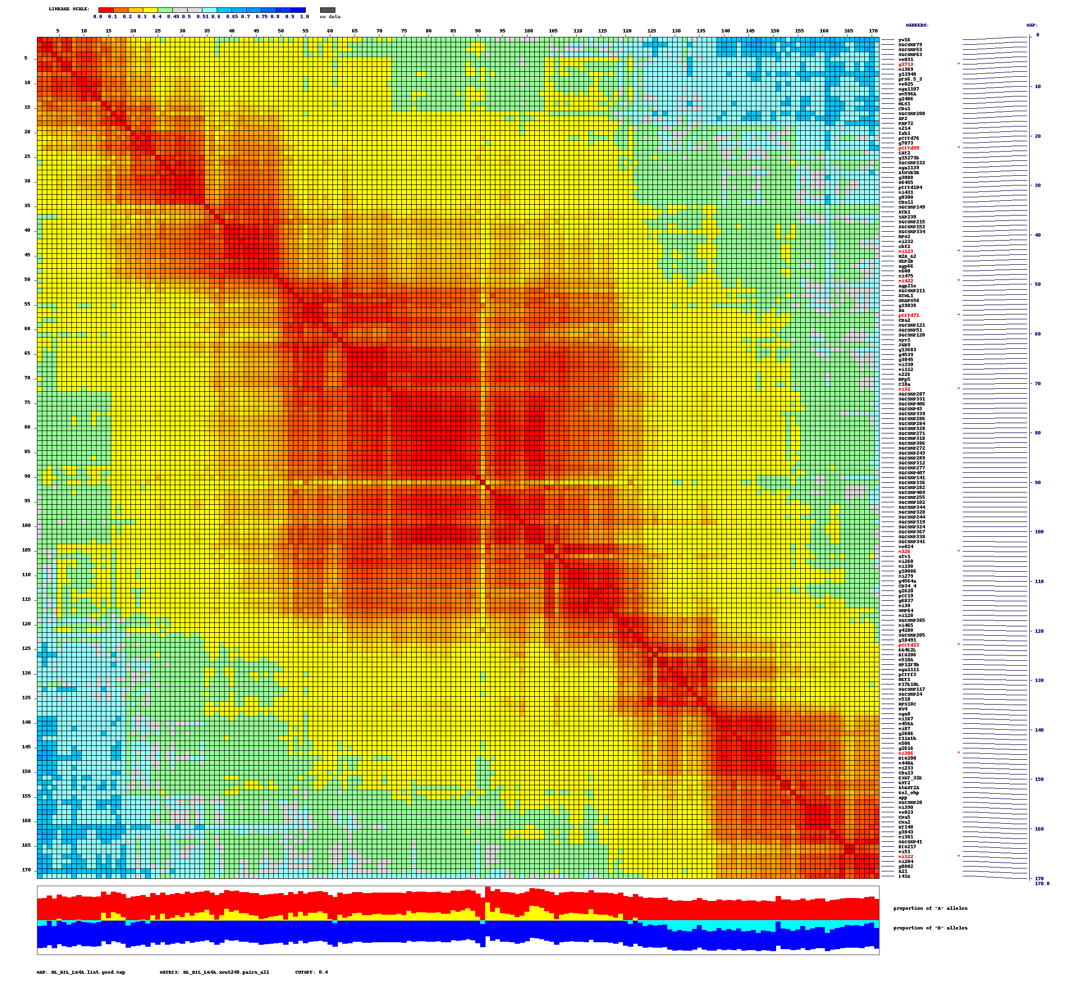
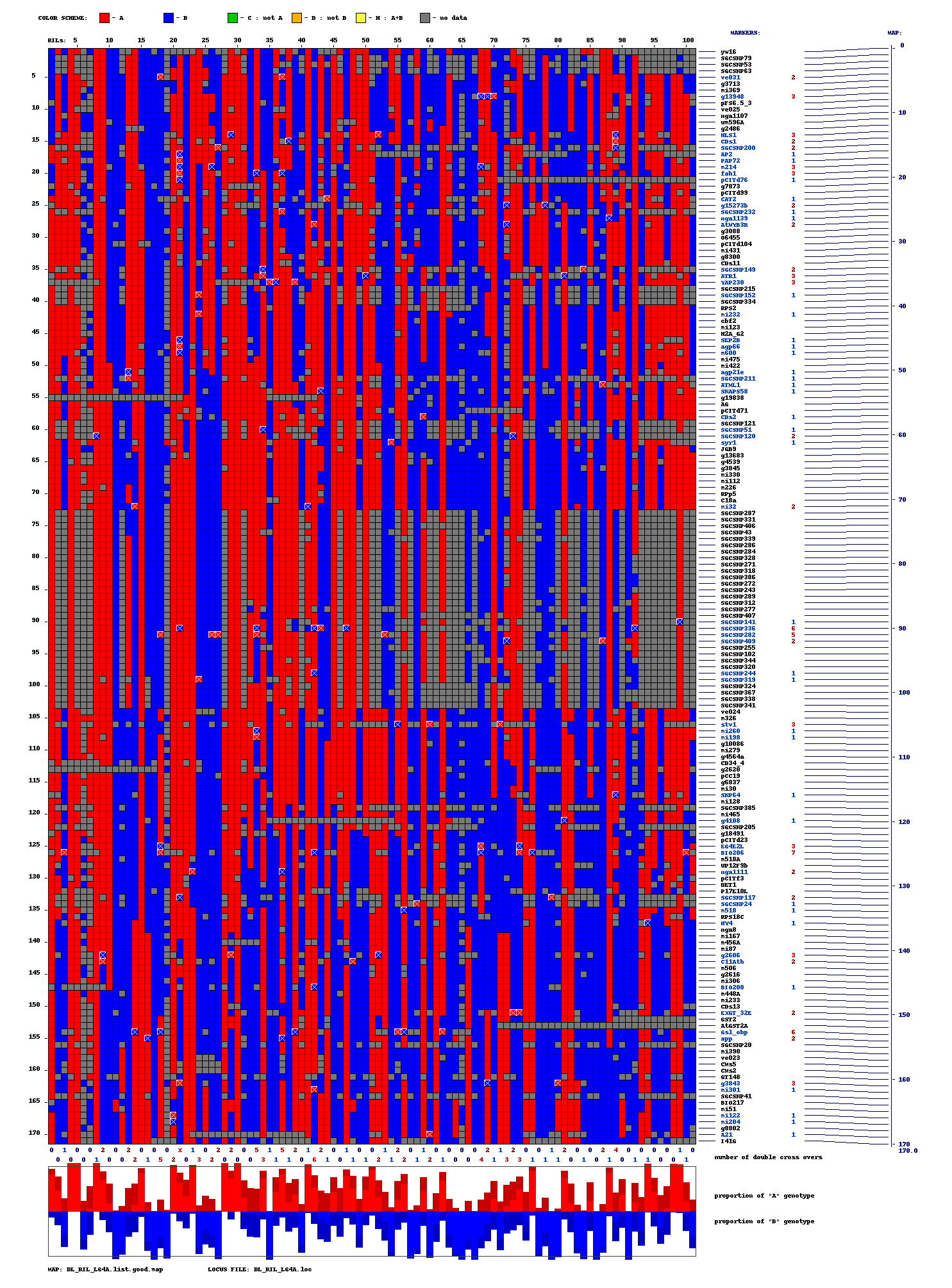
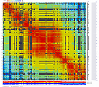
Visualization using CheckMatrix of the constructed map [ 171 'good' markers ]
(inferred linear order of markers):
Now using 'good' map with 171 markers as a frame work map with fixed order we will try to add (insert) remaining markers
[ those markers that did not fall into 'good' category during grouping (clustering) ]:
$python Python_MadMapper_V248_XDELTA_016.py
DL_RIL_LG4A.xout248.pairs_all
DL_RIL_LG4A.list
DL_RIL_LG4A.list.good.map.order
DL_RIL_LG4A.final.xdelta
4 FIXED
Output files:
1. DL_RIL_LG4A.final.xdelta.mad_map_final - final best map
2. DL_RIL_LG4A.final.xdelta.mad_map_log - log file
3. DL_RIL_LG4A.final.xdelta.mad_map_temp -
file with all best maps after each set of iterations
4. DL_RIL_LG4A.final.xdelta.mad_map_xjump - 'deltas' for each set of iterations
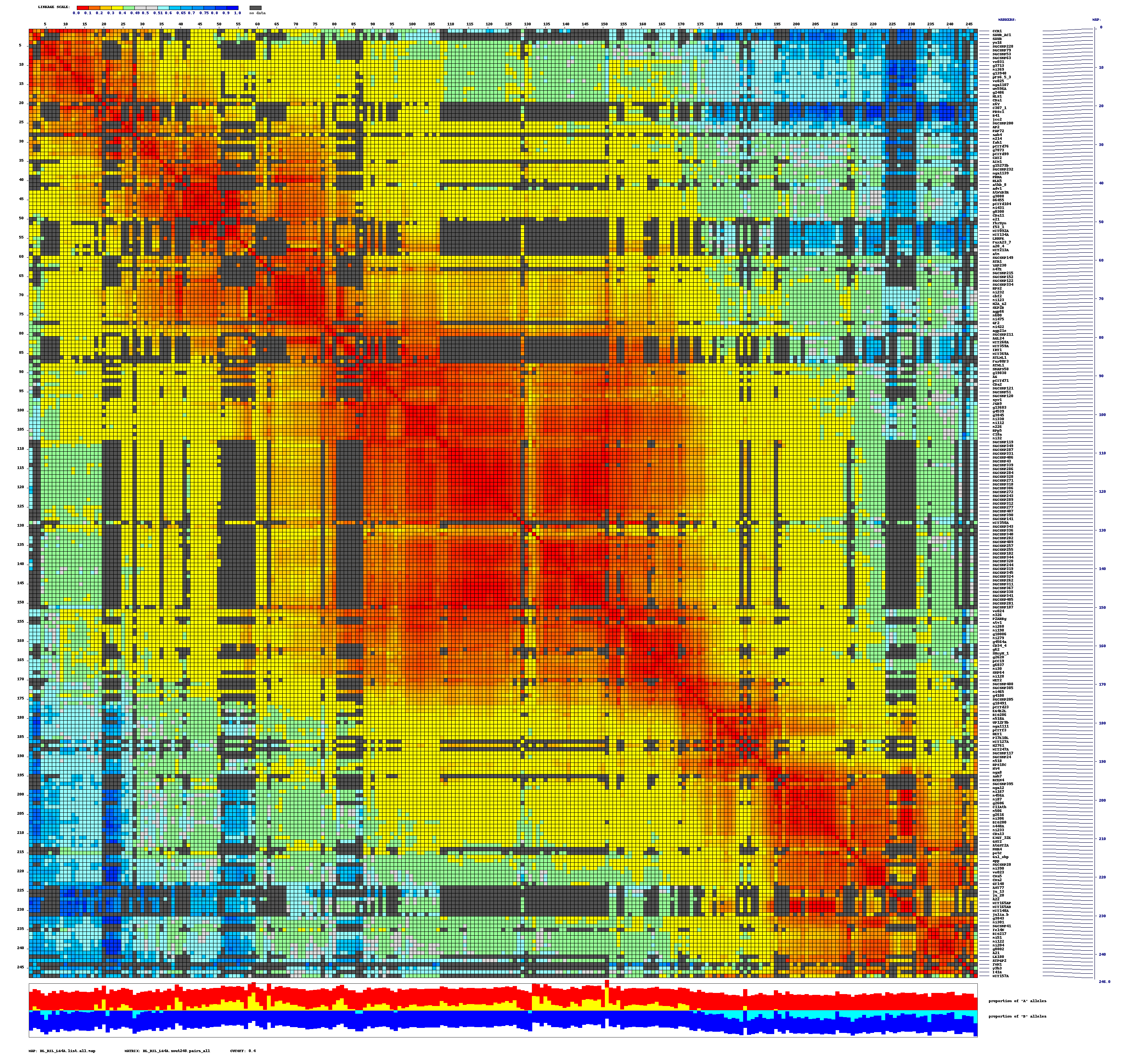
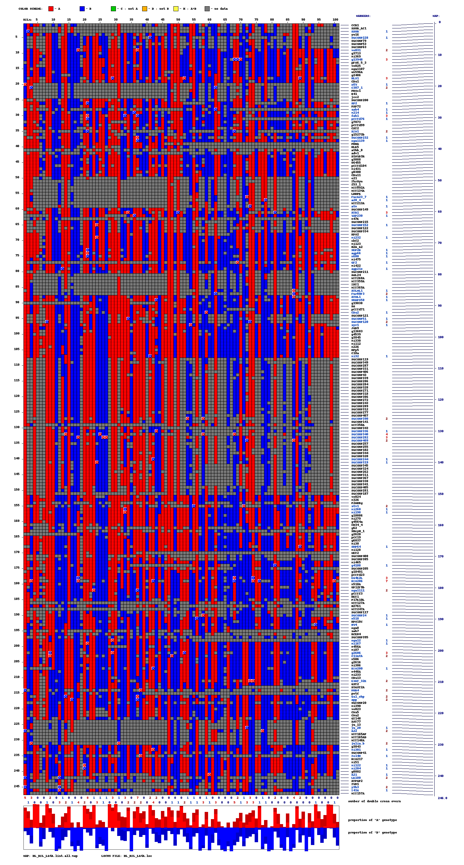
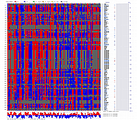
Visualization using CheckMatrix of the constructed map [ 247 all markers ]
(inferred linear order of markers):
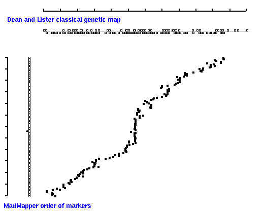
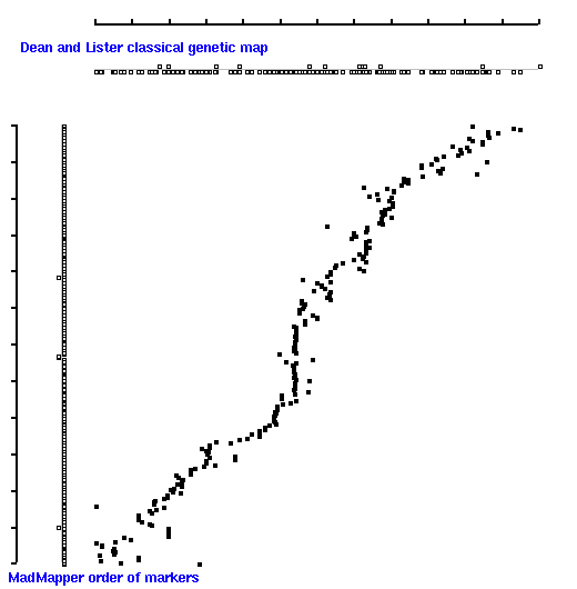
We can generate diagonal 2D dot-plots to compare linear order of markers inferred by MadMapper
to the order of markers on 'classical' genetic map constructed by Lister and Dean using MapMaker:
Dot plot of 'classical' map (X axis) versus 'good' map [ 171 markers ] generated by MadMapper (Y axis)
Dot plot of 'classical' map (X axis) versus 'all' map [ 247 markers ] generated by MadMapper (Y axis)
Images were generated using
GenomePixelizer 2D Plotter
and TwoMaps2GenoPix_002.py script.
Note, that 'classical' map displays positions of markers according to their map distances;
'madmap' displays just a relative order of markers [ without real map distances ].
Diagonal 2D dot plot indicates that the linear order of markers derived by MadMapper is
in good correlation with the order of markers derived by MapMaker.
High quality markers [ 'good' 171 set ] produces better map compare to 'all' [ 247 ] marker set.
Optimization of MadMapper approach and improvement of algorithms behind the program are
next steps of this work.
NEW! (January 14 2006)
In the latest version of MadMapper_V248_XDELTA_024 (#24) shuffle [ or ripple ]
procedure was implemented allowing re-arrangement of markers within sliding window:
Python_MadMapper_V248_XDELTA_024.py
Genetic_Map_MadMapper_Arabidopsis.html
web page describes the usage of
Python_MadMapper_V248_XDELTA_024.py
with shuffle option on Arabidopsis genetic map as an example.
CURRENT WORKING VERSIONS OF MadMapper_RECBIT and MadMapper_XDELTA:
Python_MadMapper_V248_RECBIT_012NR.py
Python_MadMapper_V248_XDELTA_115.py
Python_MadMapper_V248_XDELTA_116.py - minor bug fixes
Python_MadMapper_V248_XDELTA_119.py - can choose clolumn in matrix file with pairwise data; 'check_map' new function; minor bug fixes
example of usage MadMapper/CheckMatrix suite to construct
high-density genetic map of Arabidopsis thaliana
using Affymetrix microarray SFP genotyping data
POSTERS AND PRESENTATIONS:
AKozik_SanDiego_PAG_14_Poster.ppt -
download poster with MadMapper presentation at PAG-14 meeting
AKozik_SanDiego_PAG_14_Presentation.ppt -
dowload MadMapper presentation at PAG-14 meeting
AKozik_Poster_MadMapper_023_L.ppt - Details about MadMapper Usage
email to: akozik@atgc.org Alexander Kozik
last modified October 03 2006